Metadata
aliases: []
shorthands: {}
created: 2022-07-11 11:10:07
modified: 2022-07-11 11:39:58
In this method, we also assume that the shear zone is perpendicular to the
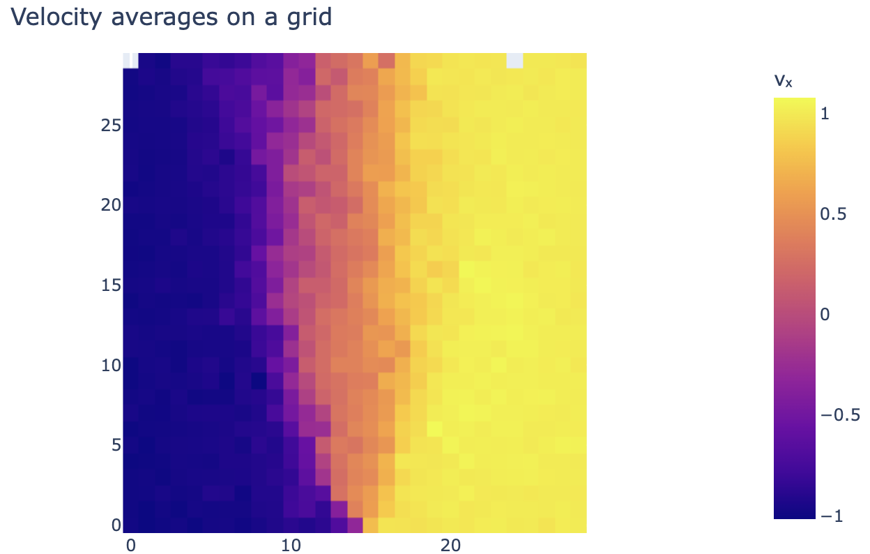
This is a simpler method for approximating the shear zone in granular materials, where we use a grid to evaluate the needed quantities.
At first, we average out the
zmin = np.min(coords[:, 2])
zmax = np.max(coords[:, 2])
xmin = -2
xmax = 2
ymin = -2
ymax = 2
effecrive_radius = (a*b*c)**(1/3)

girdres_y = int((ymax - ymin) / effecrive_radius)
girdres_z = int((zmax - zmin) / effecrive_radius)
grid_vels = np.zeros((girdres_y, girdres_z), dtype="float64")
grid_counts = np.zeros((girdres_y, girdres_z), dtype="float64")

for i in range(len(coords)):
    cs = coords[i]
    v = vs[i]
    y = int((cs[1] - ymin) / effecrive_radius)
    z = int((cs[2] - zmin) / effecrive_radius)
    if y >= girdres_y or z >= girdres_z or y < 0 or z < 0:
        continue
    grid_vels[y, z] += v[0]
    grid_counts[y, z] += 1
grid_vels /= grid_counts
Where we set the resolution of the grid according to the size of the particles involved.
We can plot this grid using imshow of plotly:
fig = px.imshow(grid_vels.T, origin="lower")
fig.update_layout(width=650, height=400, margin=dict(
    l=0, r=0, b=0, t=40), title="Velocity averages on a grid")
fig.update_layout(
    coloraxis_colorbar=dict(
        title="vₓ",
    ),
    scene=dict(
        xaxis=dict(range=[-2, 2],),
        yaxis=dict(range=[-2, 2],),
        zaxis=dict(range=[-0, 4],))
)
fig.show()
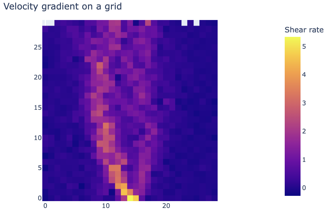
Now this gives use a great and easy to deal with representation of the velocity distribution, from which taking derivatives is easy as well:
grid_gradient_y = np.gradient(grid_vels, effecrive_radius, axis=0)
Which results in:
fig = px.imshow(grid_gradient_y.T, origin="lower")
fig.update_layout(width=650, height=400, margin=dict(
    l=0, r=0, b=0, t=40), title="Velocity gradient on a grid")
fig.update_layout(
    scene=dict(
        xaxis=dict(range=[-2, 2],),
        yaxis=dict(range=[-2, 2],),
        zaxis=dict(range=[-0, 4],)),
    coloraxis_colorbar=dict(
        title="Shear rate",
    ),
)
fig.show()
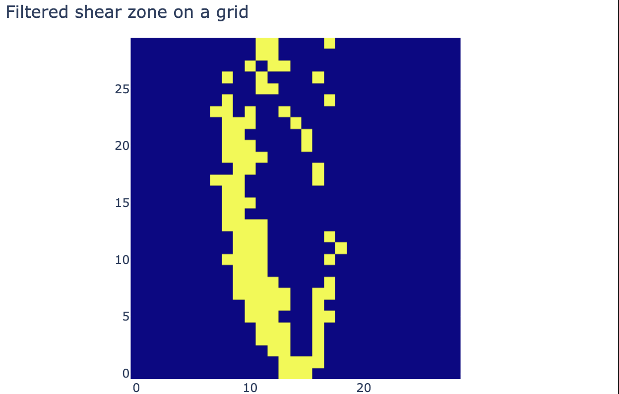
Then we can apply a filter to exclude the parts outside of the shear zone:
grid_shear_zone = np.zeros((girdres_y, girdres_z), dtype="bool")
grid_shear_zone = grid_gradient_y > 1.3
In our case this looks like:
fig = px.imshow(grid_shear_zone.T, origin="lower")
fig.update_layout(width=650, height=400, margin=dict(
    l=0, r=0, b=0, t=40), title="Filtered shear zone on a grid")
fig.update_layout(
    scene=dict(
        xaxis=dict(range=[-2, 2],),
        yaxis=dict(range=[-2, 2],),
        zaxis=dict(range=[-0, 4],)),
    coloraxis_showscale=False
)
fig.show()
But this is only applied to the grid, we also need to determine which particles fall inside the chosen grid cells:
grid_coords_y = np.array((coords[:, 1] - ymin) / effecrive_radius, dtype="int")
grid_coords_z = np.array((coords[:, 2] - zmin) / effecrive_radius, dtype="int")
coord_filter = (grid_coords_y < girdres_y) * (grid_coords_z <
                                              girdres_z) * (grid_coords_y >= 0) * (grid_coords_z >= 0)
grid_coords_y[np.invert(coord_filter)] = 0
grid_coords_z[np.invert(coord_filter)] = 0
zone_filter = grid_shear_zone[grid_coords_y, grid_coords_z]
zone_filter = zone_filter * coord_filter
Then we can scatter plot the filtered particles in 3D:
fig = go.Figure(data=[go.Scatter3d(x=coords[:, 0][zone_filter], y=coords[:, 1][zone_filter], z=coords[:, 2][zone_filter],
                                   mode='markers',
                                   marker=dict(
    size=3, color=(gradient_from_fit[zone_filter]),
    colorscale='Viridis',
    colorbar=dict(title="Approximated shear rate"),
    showscale=True))])
fig.update_layout(width=650, height=400, margin=dict(
    l=0, r=0, b=0, t=40), title="Shear zone with kernel approximation", scene_aspectmode='cube')
fig.update_layout(
    scene=dict(
        xaxis=dict(range=[-2, 2],),
        yaxis=dict(range=[-2, 2],),
        zaxis=dict(range=[-0, 4],)),
)
fig.show()
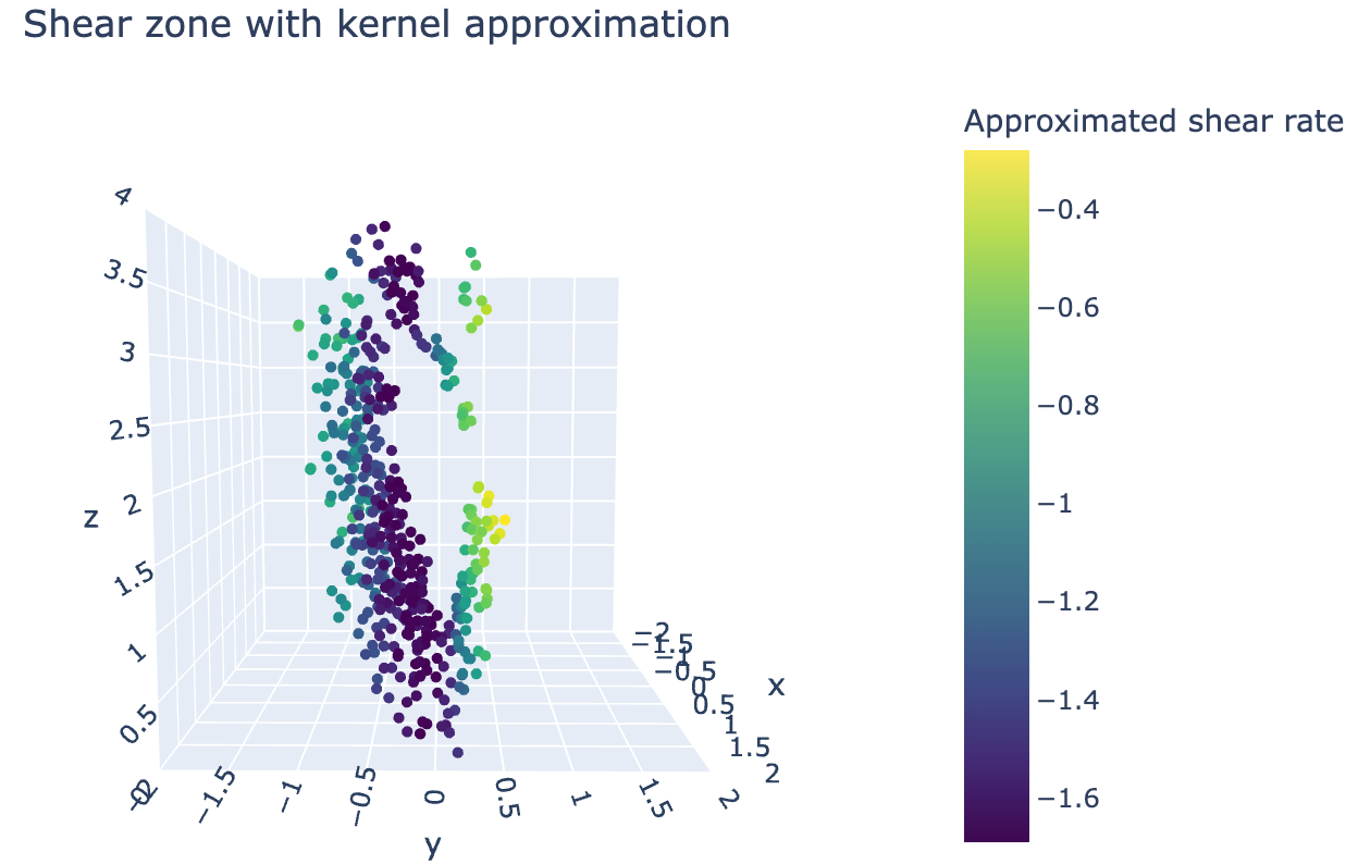
As we can see, similarly to the particle approximation method, here we also see both branches of the shear zone.